


By Garrett Seeley
In the late 1800s, mathematician Joseph Fourier analyzed complex waveforms and discovered that all waves can be represented as combinations of simpler waves. His mathematical insights made it possible to break down intricate waveforms into their fundamental frequencies and amplitudes – a process essential in many areas of science and technology.
This concept is familiar to many healthcare technology management (HTM) professionals. For instance, although we’re taught that wall AC power produces a 60 Hz sine wave, in practice the waveform is much more complex, as shown below:
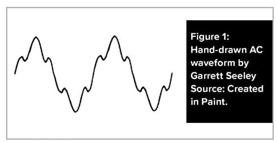
While an ideal AC sine wave appears smooth, real-world waveforms contain additional frequencies. For example, the 60 Hz AC signal is accompanied by a ripple near 100 Hz due to power grid resonance.
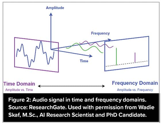
In ECG systems, filters are designed to remove both 60 Hz and 100 Hz noise. The actual AC power waveform is the sum of these components. The time domain shows the overall waveform, while the frequency domain reveals individual spikes representing specific frequencies. In essence, a complex signal can be broken down into simpler frequency components.
Imagine representing these waveforms as pixels. Frequency could be graphed along one axis, amplitude on another, positioning two pixels at different locations in the frequency domain. This process is central to imaging technologies, whether interpreting sound waves in ultrasound, radio waves in MRI or detecting slices in CT scans. Sensors (such as crystal arrays in ultrasound or coils in MRI) capture these frequencies and intensities, enabling the creation of two-dimensional images through triangulation.
In MRI, this encoded frequency data is called “K-space.” It’s detected by multiple coils, providing the basis for image reconstruction. Let’s examine how an MRI interprets radio waves from a patient.
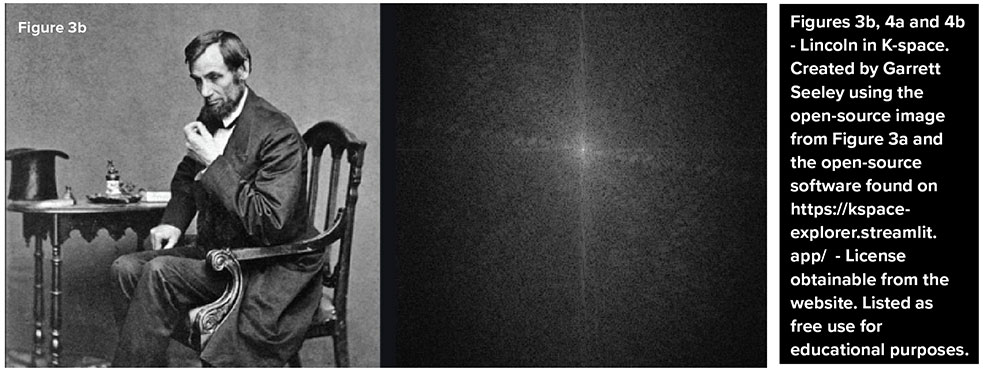
Figure 3b shows how MRI detects a picture as waveforms radiating from the center; each line represents a radio wave of variable intensity. The computer interprets images in the frequency domain as thousands of overlapping waves plotted from a central point (0,0) on an X-Y axis, extending in all directions.
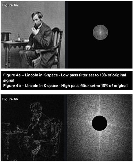 Figures 4a and 4b demonstrate the impact of removing data from different parts of K-space. Deleting the center removes structural information (Figure 4b), while removing edge data reduces image resolution (Figure 4a), as the higher frequencies are located towards the edges of k-space. Notice how the higher frequencies are used to add detail whereas the lower frequencies provide the bulk of the image structure.
These examples show how the Fourier Transform is fundamental in converting waveforms into pixel data, forming the backbone of medical imaging. The core structures of an image are derived from low-frequency waveforms, while fine diagnostic details arise from high-frequency components. Thus, a diagnostic image is the sum of waveforms transformed to their intensity and frequency and graphed on a map.
Fourier’s mathematical approach allows imaging equipment to visualize intricate biological structures, making advanced diagnostics possible.
Try kspace-explorer.streamlit.app/ to experience K-space encoding yourself!